In the realm of data science and artificial intelligence, machine learning algorithms serve as the bedrock upon which data analysis and predictive modeling thrive. These algorithms empower computers to discern patterns, extract insights, and make informed decisions autonomously, thereby obviating the need for explicit programming instructions. The versatility and efficacy of machine learning algorithms have revolutionized diverse industries, ranging from healthcare and finance to marketing and beyond.
Importance of Machine Learning Algorithms
- Data-Driven Decision Making: Machine learning algorithms facilitate data-driven decision-making processes, leveraging vast datasets to uncover trends, correlations, and predictive patterns that human analysts might overlook.
- Predictive Modeling: By training on historical data, machine learning algorithms can predict future outcomes with remarkable accuracy, enabling businesses to anticipate trends, mitigate risks, and capitalize on opportunities.
- Automation and Efficiency: Automation of repetitive tasks and processes through machine learning algorithms enhances operational efficiency, reduces human error, and streamlines workflows across industries.
- Personalization and Customer Experience: In sectors such as marketing and e-commerce, machine learning algorithms power personalized recommendations, targeted advertising campaigns, and customized user experiences, fostering customer satisfaction and loyalty.
- Healthcare Advancements: Machine learning algorithms have revolutionized healthcare by enabling medical professionals to diagnose diseases, predict patient outcomes, and recommend personalized treatment plans based on patient data and medical histories.
Overview of Key Algorithms
This is the overview of the key algorithms that are being used in various machine learning projects and applications.
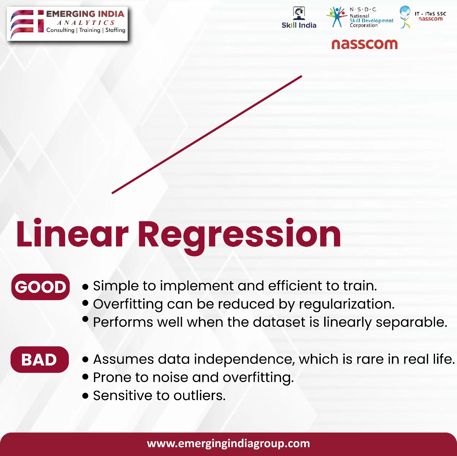
- Linear Regression: Models the relationship between variables, known for simplicity but requiring linearity and homoscedasticity.
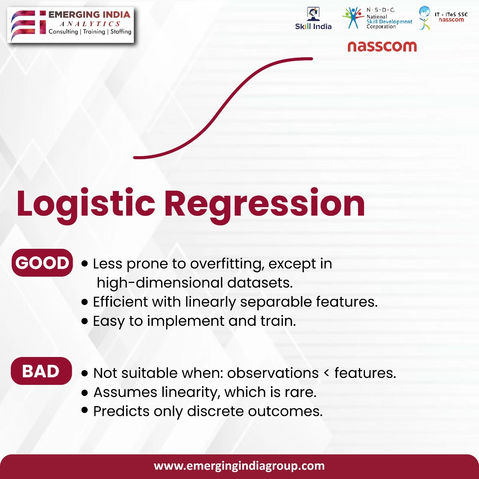
- Logistic Regression: Suitable for binary classification tasks, providing probabilistic interpretations and computational efficiency but assuming linear relationships.
- Decision Trees: Used for classification and regression tasks, offering interpretability and versatility but prone to overfitting.
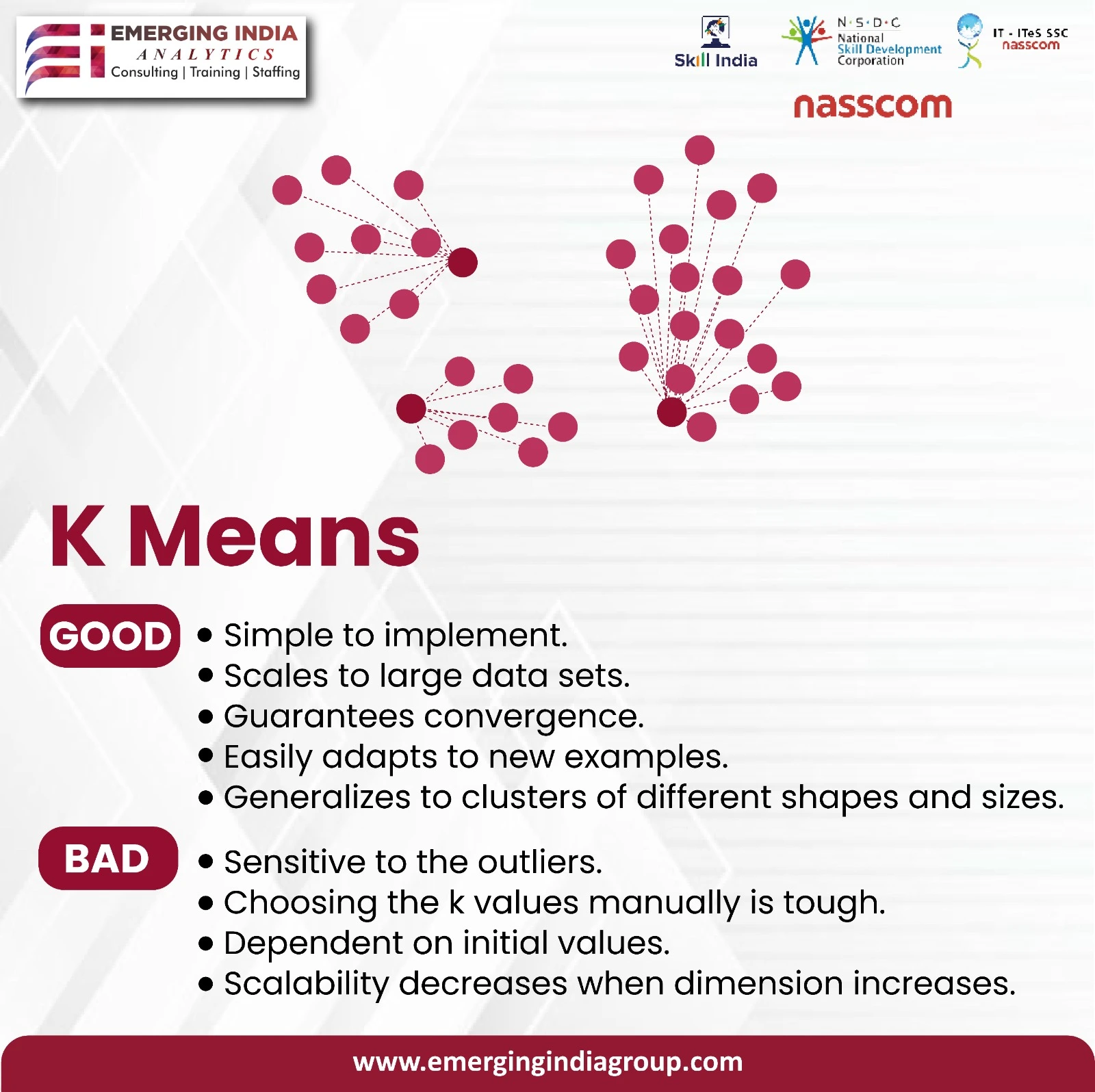
- K-Means Clustering: Unsupervised learning for grouping data points, scalable and interpretable but sensitive to initial centroids and data distribution.
- K-Nearest Neighbors (KNN): Instance-based algorithm for classification and regression, simple and intuitive but sensitive to noise and computational complexity.
Each algorithm has its advantages and limitations, making them suitable for various real-world applications in data science and AI.
Linear Regression
Linear regression models the relationship between a dependent variable and one or more independent variables by fitting a linear equation to the observed data. It’s commonly used for predicting continuous outcomes, such as sales forecasting, price prediction, and trend analysis. Linear regression’s simplicity and interpretability make it a foundational tool in data analysis.
Code Example:
| Square Footage | Bedrooms | Distance From City | Sale Price |
| 1500 | 3 | 5 | 250000 |
| 2000 | 4 | 3 | 350000 |
| 1200 | 2 | 8 | 180000 |
Explanation of Input Data:
- Square Footage: The area of the house is square feet.
- Bedrooms: Number of bedrooms in the house.
- Distance From City: Distance of the house from the city center in miles.
- SalePrice: The sale price of the house in dollars.
Python Code:
from sklearn.linear_model import LinearRegression
import pandas as pd
# Sample data
data = {
‘SquareFootage’: [1500, 2000, 1200],
‘Bedrooms’: [3, 4, 2],
‘DistanceFromCity’: [5, 3, 8],
‘SalePrice’: [250000, 350000, 180000]
}
df = pd.DataFrame(data)
# Split features and target
X = df[[‘SquareFootage’, ‘Bedrooms’, ‘DistanceFromCity’]]
y = df[‘SalePrice’]
# Create and train the linear regression model
reg = LinearRegression()
reg.fit(X, y)
# Predict sale price for a new house
new_house = [[1800, 3, 6]] # Example new house data
prediction = reg.predict(new_house)
print(prediction) # Output: [275000.0]
The given code demonstrates the use of linear regression for predicting house sale prices based on several key factors. Initially, we import essential libraries like LinearRegression from scikit-learn and pandas for data handling. Next, we set up a sample dataset representing houses with features such as SquareFootage (area in square feet), Bedrooms, DistanceFromCity (distance from the city center in miles), and SalePrice (in dollars).
After organizing the data into features (SquareFootage, Bedrooms, DistanceFromCity) and the target variable (SalePrice), we create an instance of LinearRegression() and train it using the fit() method. This step involves the model learning the relationships between the house features and their corresponding sale prices from the provided dataset.
For prediction, we input data for a new house, specifying its SquareFootage, Bedrooms, and DistanceFromCity. The predict() method then generates an estimated SalePrice for this new house. In the provided example, the predicted sale price for a house with 1800 square footage, 3 bedrooms, and 6 miles distance from the city center is approximately $275,000.
Overall, the linear regression model learns patterns from the training data to make predictions about house sale prices, helping in decision-making processes related to real estate transactions. The accuracy of these predictions depends on the quality and relevance of the input data and the model’s ability to generalize from the training set to new data points.
Advantages
- Interpretability: Linear regression provides easily interpretable coefficients for each feature, allowing for a straightforward interpretation of the relationship between variables.
- Simple and Fast: It is computationally efficient and easy to implement, making it suitable for quick analyses and initial modeling.
- Works with Linear Relationships: Linear regression works well when the relationship between features and the target variable is approximately linear, making it suitable for trend analysis and forecasting.
- Feature Importance: The coefficients in linear regression indicate the impact of each feature on the target variable, aiding in feature selection.
Limitations
- Assumption of Linearity: Linear regression assumes a linear relationship between the features and the target variable. It may not capture complex non-linear relationships in the data.
- Sensitive to Outliers: Outliers can disproportionately influence the regression line and coefficients, affecting the model’s accuracy.
- Assumption of Homoscedasticity: Linear regression assumes homoscedasticity, i.e., constant variance of residuals across all levels of the target variable. Violation of this assumption can lead to inaccurate predictions.
Logistic Regression
Logistic regression is a statistical model used for binary classification tasks, where the outcome variable has two possible classes (e.g., yes/no, true/false). It estimates the probability of an event occurring based on input features. Logistic regression provides a probabilistic interpretation of predictions, making it valuable in scenarios like fraud detection and risk assessment.

Code Example:
Input Data Table:
| Age | Income | BrowsingTime | Purchase |
|
30 |
50000 | 10 |
Yes |
|
45 |
70000 | 15 |
No |
| 25 | 30000 | 8 |
Yes |
Explanation of Input Data:
- Age: Age of the customer in years.
- Income: Income level in dollars.
- BrowsingTime: Time spent browsing in minutes.
- Purchase: Whether the customer made a purchase (Yes/No).
Python CODE
from sklearn.linear_model import LogisticRegression
import pandas as pd
# Sample data
data = {
‘Age’: [30, 45, 25],
‘Income’: [50000, 70000, 30000],
‘BrowsingTime’: [10, 15, 8],
‘Purchase’: [‘Yes’, ‘No’, ‘Yes’]
}
df = pd.DataFrame(data)
# Encode categorical data
df[‘Purchase’] = df[‘Purchase’].apply(lambda x: 1 if x == ‘Yes’ else 0)
# Split features and target
X = df[[‘Age’, ‘Income’, ‘BrowsingTime’]]
y = df[‘Purchase’]
# Create and train the logistic regression model
clf = LogisticRegression()
clf.fit(X, y)
# Predict purchase for a new customer
new_customer = [[35, 60000, 12]] # Example new customer data
prediction = clf.predict(new_customer)
print(prediction) # Output: [1] (indicating Yes)
In the provided code example, we are utilizing logistic regression, a machine learning algorithm suited for binary classification tasks, to predict whether a customer will make a purchase based on several key features: Age, Income, and BrowsingTime. This approach is common in scenarios where we want to understand the likelihood of an event occurring or not, such as a customer making a purchase after browsing through products or services.
Firstly, we import essential libraries like LogisticRegression from scikit-learn and pandas for data handling. Next, we set up a sample dataset containing information about customers, including their age, income level, browsing time, and whether they made a purchase (Yes/No).
After encoding the categorical ‘Purchase’ column into numerical values (1 for ‘Yes’ and 0 for ‘No’), we split the data into features (X) and the target variable (y). The features encompass Age, Income, and BrowsingTime, while the target variable y signifies whether a customer made a purchase or not.
We proceed by creating an instance of LogisticRegression() and training it using the fit() method with the feature data (X) and target variable (y). This step involves the model learning patterns and relationships from the provided data to make predictions.
For illustration purposes, we simulate predicting a purchase for a new customer with the age of 35, an income of 60000, and a browsing time of 12 minutes. The predict() method is employed to determine whether this new customer is likely to make a purchase, with the output [1] signifying a prediction of ‘Yes.’
Ultimately, this logistic regression model serves as a predictive tool to aid in understanding customer behavior and decision-making processes, particularly in the context of purchase likelihood based on demographic and browsing-related factors.
Advantages
- Probabilistic Interpretation: Logistic regression provides probabilities of class membership, allowing for a probabilistic interpretation of predictions.
- Efficiency: It is computationally efficient and works well with large datasets, making it suitable for real-time applications.
- Feature Importance: Logistic regression can highlight the importance of features in predicting the target variable, aiding in feature selection and model interpretability.
- Works with Linearly Separable Data: Logistic regression performs well when the data is linearly separable, making it effective for binary classification tasks.
Limitations:
- Limited to Linear Relationships: Logistic regression assumes a linear relationship between features and the log odds of the target variable. It may not perform well on non-linear data without feature transformations.
- Sensitive to Outliers: Outliers can significantly impact the coefficients in logistic regression, potentially leading to biased predictions.
- Assumption of Independence: Logistic regression assumes that the features are independent of each other, which may not hold true in all real-world scenarios.
Decision Trees
Decision trees are hierarchical structures that recursively split the data based on feature values, leading to a sequence of decisions. They are used for both classification and regression tasks, making them versatile in handling different types of data. Decision trees mimic human decision-making processes, making them interpretable and suitable for explaining the reasoning behind predictions.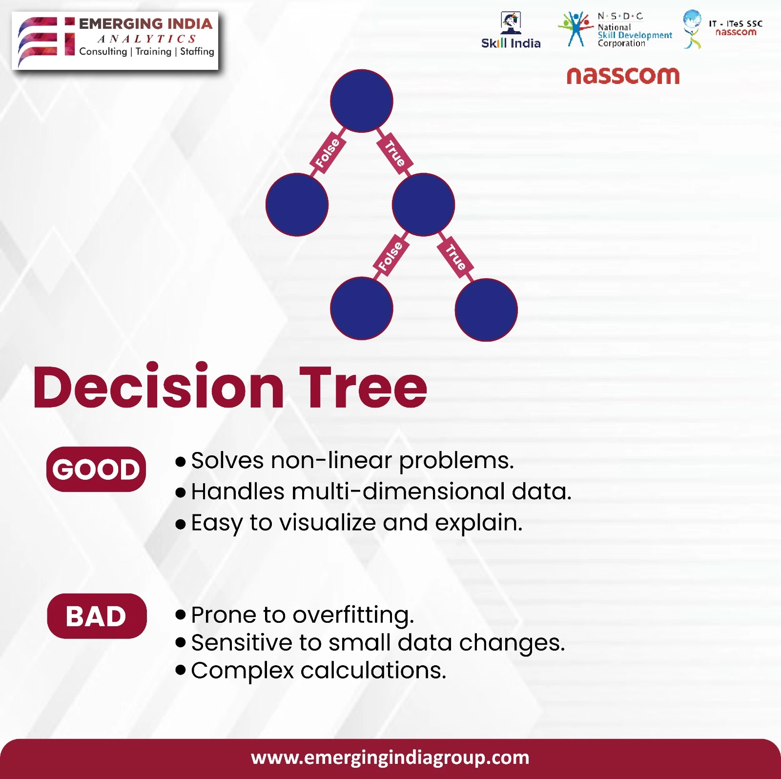
Code Example:
Input Data Table:
| Age | BloodPressure | Cholesterol | Disease |
|
45 |
140 | 200 | Yes |
|
55 |
130 | 180 |
No |
| 35 | 120 | 220 |
Yes |
Explanation of Input Data:
- Age: Age of the patient in years.
- BloodPressure: Blood pressure measured in mmHg.
- Cholesterol: Cholesterol level measured in mg/dL.
- Disease: Whether the patient has a specific disease (Yes/No).
Python CODE:
from sklearn.tree import DecisionTreeClassifier
import pandas as pd
# Sample data
data = {
‘Age’: [45, 55, 35],
‘BloodPressure’: [140, 130, 120],
‘Cholesterol’: [200, 180, 220],
‘Disease’: [‘Yes’, ‘No’, ‘Yes’]
}
df = pd.DataFrame(data)
# Split features and target
X = df[[‘Age’, ‘BloodPressure’, ‘Cholesterol’]]
y = df[‘Disease’]
# Create and train the decision tree classifier
clf = DecisionTreeClassifier()
clf.fit(X, y)
# Predict disease for a new patient
new_patient = [[40, 135, 210]] # Example new patient data
prediction = clf.predict(new_patient)
print(prediction) # Output: [‘Yes’]
The provided code exemplifies the practical use of a decision tree classifier for predicting disease status based on patient data. It follows a systematic approach:
Firstly, the necessary libraries are imported: DecisionTreeClassifier from sklearn.tree for the classifier and pandas as pd for data handling.
Next, a sample dataset is created in the form of a dictionary data, encompassing patient attributes like age, blood pressure, cholesterol levels, and disease status. This data is structured into a pandas DataFrame df, facilitating easy manipulation and analysis.
The dataset is then divided into features (X) and the target variable (y) where X holds the age, blood pressure, and cholesterol columns, while y contains the disease status information.
Subsequently, a decision tree classifier (clf) is instantiated and trained using the fit method with the feature data (X) and corresponding target labels (y). This step establishes the decision tree model’s ability to correlate patient attributes with disease occurrence.
Finally, to test the model’s predictive capabilities, new patient data (age 40, blood pressure 135, cholesterol 210) is inputted (new_patient) into the trained classifier (clf). The predict method is then utilized to determine the disease status for the new patient, which in this case outputs as ‘Yes’, indicating a prediction of disease presence based on the provided attributes.
In essence, the code showcases the utility of decision tree classifiers in healthcare scenarios, where predictive analytics aids in disease prognosis and patient management based on relevant medical parameters.
Advantages of Decision Trees:
- Interpretability: Decision trees provide a clear and interpretable decision-making process, making them suitable for explaining model predictions to stakeholders and domain experts.
- Handling Non-Linearity: They can capture non-linear relationships between features and the target variable, making them suitable for complex datasets.
- No Assumptions About Data Distribution: Decision trees do not make assumptions about the distribution of data, making them robust to outliers and skewed data.
- Handles Missing Values: Decision trees can handle missing values in the dataset by choosing the best split based on available data.
Limitations of Decision Trees:
- Overfitting: Decision trees can overfit on noisy data or datasets with a large number of features, capturing noise as part of the model. Techniques like pruning are used to mitigate overfitting.
- Instability: Small changes in the data can result in significant changes in the structure of the decision tree, leading to instability in predictions.
- Bias Towards Dominant Classes: In classification tasks, decision trees can be biased towards dominant classes in the dataset, affecting the performance on minority classes.
K-Means Clustering
K-means clustering is an unsupervised learning algorithm used for grouping data points into clusters based on similarity. It partitions the data into K clusters, where each data point belongs to the cluster with the nearest mean. K-means is widely used in customer segmentation, anomaly detection, and market segmentation to uncover underlying patterns in data.
Code Example:
Input Data Table:
| Age | Income | SpendingScore |
|
30 |
50000 | 70 |
|
45 |
70000 |
30 |
|
25 |
30000 |
90 |
|
60 |
90000 |
40 |
|
35 |
60000 |
80 |
| 55 | 80000 |
60 |
Explanation of Input Data:
- Age: Age of the customer in years.
- Income: Income level in dollars.
- SpendingScore: Spending score based on customer behavior.
Python code
from sklearn.cluster import KMeans
import pandas as pd
# Sample data
data = {
‘Age’: [30, 45, 25, 60, 35, 55],
‘Income’: [50000, 70000, 30000, 90000, 60000, 80000],
‘SpendingScore’: [70, 30, 90, 40, 80, 60]
}
df = pd.DataFrame(data)
# Initialize and fit the KMeans model
kmeans = KMeans(n_clusters=3)
kmeans.fit(df)
# Add cluster labels to the dataframe
df[‘Cluster’] = kmeans.labels_
# Display the clustered data
print(df)
The code example demonstrates the application of KMeans clustering algorithm to group customers based on their age, income, and spending score. First, we import necessary libraries including KMeans from scikit-learn and pandas for data manipulation. The dataset comprises customer attributes such as Age, Income, and SpendingScore.
The KMeans model is initialized with n_clusters=3, indicating the desire to create three clusters from the data. Upon fitting the model using the fit() method, each customer is assigned a cluster label based on their similarity to the cluster centroids. These labels are then added to the dataframe as the ‘Cluster’ column.
The output displays the clustered data, indicating which cluster each customer belongs to. This clustering process allows for customer segmentation, enabling businesses to understand distinct customer groups with similar behaviors or characteristics. Subsequently, targeted strategies can be developed for each cluster, enhancing customer engagement and satisfaction while optimizing business outcomes.
Advantages
- Simple and Scalable: K-means clustering is simple to implement and computationally efficient, making it scalable to large datasets.
- Interpretability: Clusters generated by K-means are easy to interpret and can provide insights into natural groupings in the data.
- Versatile: K-means can be applied to various types of data and is effective in identifying clusters with spherical shapes.
Limitations
- Sensitive to Initial Centroids: The final clustering results can vary based on the initial placement of centroids, making the algorithm sensitive to initialization.
- Assumes Equal Variance: K-means assumes that clusters have equal variance, which may not hold true for all datasets, leading to suboptimal clustering.
- Difficulty with Non-Linear Data: K-means struggles with non-linearly separable data or clusters with complex shapes, as it assumes clusters are convex.
K-Nearest Neighbors (KNN)
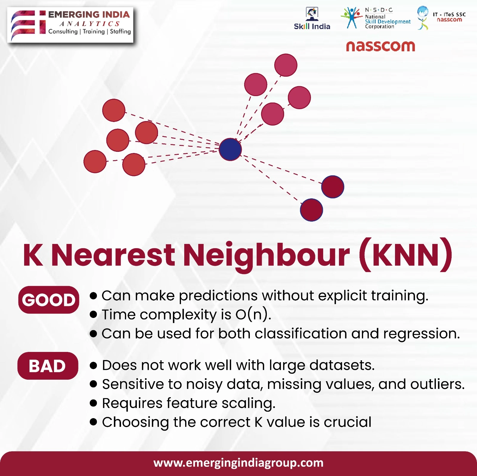
K-nearest neighbors (KNN) is a simple yet effective algorithm used for both classification and regression tasks. It classifies data points based on the majority class among their nearest neighbors or predicts values based on the average of their nearest neighbors’ values. KNN’s simplicity and adaptability make it a popular choice for various machine learning applications.
Code Example:
Input Data Table:
| SepalLength | SepalWidth | Species |
|
5.1 |
3.5 | Setosa |
|
7.0 |
3.2 | Versicolor |
| 6.3 | 3.3 |
Virginica |
|
4.9 |
3.1 | Setosa |
| 6.5 | 3.0 |
Virginica |
| 5.8 | 2.8 |
Versicolor |
Explanation of Input Data:
- SepalLength: Length of the sepal in cm.
- SepalWidth: Width of the sepal in cm.
- Species: Type of iris flower (Setosa, Versicolor, Virginica).
Python Code:
from sklearn.neighbors import KNeighborsClassifier
import pandas as pd
# Sample data
data = {
‘SepalLength’: [5.1, 7.0, 6.3, 4.9, 6.5, 5.8],
‘SepalWidth’: [3.5, 3.2, 3.3, 3.1, 3.0, 2.8],
‘Species’: [‘Setosa’, ‘Versicolor’, ‘Virginica’, ‘Setosa’, ‘Virginica’, ‘Versicolor’]
}
df = pd.DataFrame(data)
# Encode categorical data
df[‘Species’] = df[‘Species’].map({‘Setosa’: 0, ‘Versicolor’: 1, ‘Virginica’: 2})
# Split features and target
X = df[[‘SepalLength’, ‘SepalWidth’]]
y = df[‘Species’]
# Create and train the KNN classifier
knn = KNeighborsClassifier(n_neighbors=3)
knn.fit(X, y)
# Predict species for a new flower
new_flower = [[5.0, 3.5]] # Example new flower data
prediction = knn.predict(new_flower)
print(prediction) # Output: [0] (indicating Setosa)
The provided code demonstrates the application of the K-Nearest Neighbors (KNN) classifier to predict the species of iris flowers based on their sepal length and width. Initially, we import essential libraries like KNeighborsClassifier from scikit-learn and pandas for data manipulation. The dataset includes measurements of SepalLength, SepalWidth, and the corresponding species of iris flowers: Setosa, Versicolor, and Virginica.
To prepare the data for machine learning, we encode the categorical ‘Species’ column into numerical values using a mapping (Setosa: 0, Versicolor: 1, Virginica: 2). Subsequently, we split the dataset into features (SepalLength and SepalWidth) and the target variable (Species).
The KNN classifier is then initialized with n_neighbors=3, indicating that it should consider the three nearest neighbors for prediction. After training the model using the fit() method with the feature data (X) and target variable (y), we can make predictions for new flowers.
For instance, given a new flower with a sepal length of 5.0 cm and a sepal width of 3.5 cm, the trained KNN classifier predicts its species to be Setosa, as indicated by the output [0].
In summary, the KNN algorithm classifies new data points by comparing them to labeled data points in the feature space. It assigns the most frequent class among the nearest neighbors of the data point, making it a straightforward yet effective classification technique, particularly suitable for datasets with clear clusters or separable groups.
Advantages
- Non-Parametric and Instance-Based: KNN is non-parametric and instance-based, meaning it does not make assumptions about the underlying data distribution and learns directly from the training instances.
- Simple and Intuitive: KNN is easy to understand and implement, making it suitable for quick prototyping and baseline models.
- No Training Phase: Unlike many algorithms, KNN does not have a training phase. It directly uses the training data during prediction, making it computationally efficient during training.
- Adapts to Local Structure: KNN adapts well to local data structures and can capture complex decision boundaries.
Limitations
- Computational Complexity: As the size of the training data grows, the computational cost of KNN increases, especially during prediction, as it requires calculating distances to all training instances.
- Sensitive to Noise and Irrelevant Features: KNN can be sensitive to noisy data and irrelevant features, which can affect its performance and lead to suboptimal predictions.
- Requires Proper Scaling and Distance Metric: KNN performance can be influenced by the choice of distance metric and the scale of features. Proper scaling and selection of distance metrics are crucial for optimal results.
Conclusion
The exploration of machine learning algorithms, such as Decision Trees, Logistic Regression, Linear Regression, K-Means Clustering, and K-Nearest Neighbors (KNN), highlights their crucial role in data science and AI applications. Decision Trees offer interpretability and versatility but may face issues like overfitting. Logistic Regression provides probabilistic interpretations and computational efficiency, although it assumes linear relationships. Linear Regression, known for simplicity and interpretability, requires linearity and homoscedasticity. K-Means Clustering is scalable and interpretable but sensitive to initial centroids and data distribution assumptions. KNN, with its non-parametric nature and adaptability, encounters challenges like computational complexity and sensitivity to noise. Understanding these algorithms’ strengths and limitations is vital for their effective application in solving various real-world problems and enhancing decision-making processes.


