.“Skewness essentially measures the symmetry of the distribution, while kurtosis determines the heaviness of the distribution tails.”
The understanding shape of data is a crucial action. It helps to understand where the most information is lying and analyze the outliers in a given data. In this article, we’ll learn about the shape of data, the importance of skewness The types of skewness analyze the shape of data in the given dataset.
Skewness
If the values of a specific independent variable (feature) are skewed, depending on the model, skewness may violate model assumptions or may reduce the interpretation of feature importance.
In statistics, skewness is a degree of asymmetry observed in a probability distribution that deviates from the symmetrical normal distribution (bell
curve) in a given set of data.
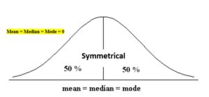
The normal distribution helps to know a skewness. When we talk about normal distribution, data symmetrically distributed. The symmetrical distribution has zero skewness as all measures of a central tendency lies in the middle.

When data is symmetrically distributed, the left-hand side, and right-hand side, contain the same number of observations. (If the dataset has 90 values, then the left-hand side has 45 observations, and the right-hand side has 45 observations.). But, what if not symmetrical distributed? That data is called asymmetrical data, and that time skewness
comes into the picture.
Types of skewness
- Positive skewed or right-skewed
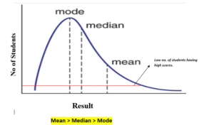
In statistics, a positively skewed distribution is a sort of distribution where, unlike symmetrically distributed data where all measures of the central tendency (mean, median, and mode) equal each other, with positively skewed data, the measures are dispersing, which means Positively Skewed Distribution is a type of distribution where the mean, median, and mode of the distribution are positive rather than negative or zero.

In positively skewed, the mean of the data is greater than the median (a large number of data-pushed on the right-hand side). In other words, the results are bent towards the lower side. The mean will be more than the median as the median is the middle value and mode is always the highest value
The extreme positive skewness is not desirable for distribution, as a high level of skewness can cause misleading results. The data transformation tools are helping to make the skewed data closer to a normal distribution. For positively skewed distributions, the famous transformation is the log transformation. The log transformation proposes the calculations of the natural logarithm for each value in the dataset.
- Negative skewed or left-skewed
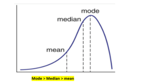
A negatively skewed distribution is the straight reverse of a positively skewed distribution. In statistics, negatively skewed distribution refers to the distribution model where more values are plots on the right side of the graph, and the tail of the distribution is spreading on the left side.
In negatively skewed, the mean of the data is less than the median (a large number of data-pushed on the left-hand side). Negatively Skewed Distribution is a type of distribution where the mean, median, and mode of the distribution are negative rather than positive or zero.

Median is the middle value, and mode is the highest value, and due to unbalanced distribution median will be higher than the mean.
Calculate the skewness coefficient of the sample
Pearson’s first coefficient of skewness
Subtract a mode from a mean, then divides the difference by standard deviation.
As Pearson’s correlation coefficient differs from -1 (perfect negative linear relationship) to +1 (perfect positive linear relationship), including a value of 0 indicating no linear relationship, When we divide the covariance values by the standard deviation, it truly scales the value down to a limited range of -1 to +1. That accurately the range of the correlation values.
Pearson’s first coefficient of skewness is helping if the data present high mode. But, if the data have low mode or various modes, Pearson’s first coefficient is not preferred, and Pearson’s second coefficient may be superior, as it does not rely on the mode.
Pearson’s second coefficient of skewness
Multiply the difference by 3, and divide the product by standard deviation.

If the skewness is between -0.5 & 0.5, the data are nearly symmetrical.
If the skewness is between -1 & -0.5 (negative skewed) or between 0.5 & 1(positive skewed), the data are slightly skewed.
If the skewness is lower than -1 (negative skewed) or greater than 1 (positive skewed), the data are extremely skewed.
Summary
The skewness is a measure of symmetry or asymmetry of data distribution Data can be positive-skewed (data-pushed towards the right side) or negative-skewed (data-pushed towards the left side).
When data skewed, the tail region may behave as an outlier for the statistical model, and outliers unsympathetically affect the model’s performance especially regression-based models. Some statistical models are hardy to outliers like Tree-based models, but it will limit the possibility to try other models. So there is a necessity to transform the skewed data to close enough to a Normal distribution.


